Computer Vision Algorithms
Eight MATLAB exercise sets that implement the maths behind computer vision from first principles: camera geometry, gradients and edges, Hough lines, Fourier analysis, SVD, histogram processing and motion detection. The biggest is an industrial door-gap detector.
Door-gap detection
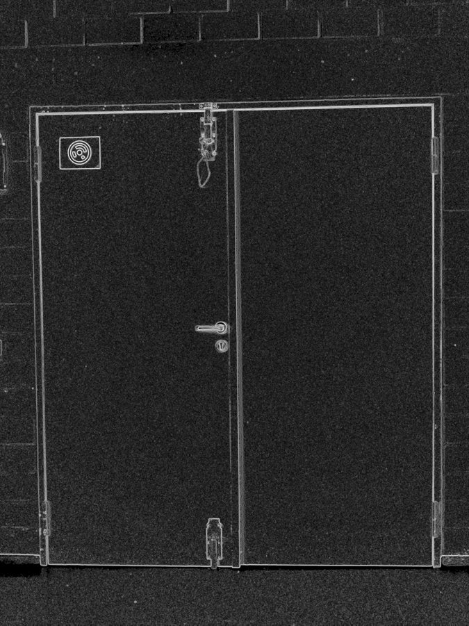
Find the thin rectangular gap between a door and its frame, an industrial inspection task. A gap shows up as a light → dark → light transition: a negative gradient right next to a positive one. These four images are the actual stages, rendered from the solution files my script saved.


From pixels to edges
- Pre-processing: grayscale,
imadjust, then a separable binomial low-pass filter[1 4 6 4 1]/16along x and then y. - Optimised Sobel kernels (Scharr-style weights
[-3 0 3; -10 0 10; -3 0 3]/32), which are more rotation-invariant than plain Sobel. - Separate masks for positive and negative gradients, each thresholded at
0.5 × mean(|∇|), cleaned withimopenand grown withimdilate. - The AND of the negative and positive masks isolates symmetric transitions. A
[-1 2 -1]filter sharpens them.
From edges to geometry
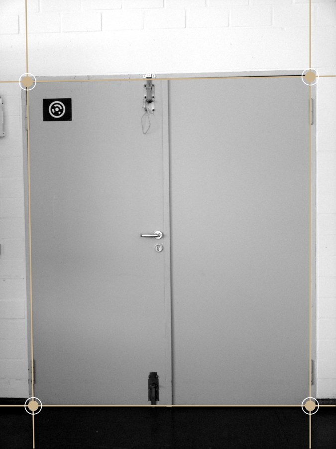
- The Hough transform runs separately on the vertical and horizontal candidate maps.
houghpeakskeeps up to 5 peaks above 30% of the maximum, and longFillGap/MinLengthvalues keep only full door edges. - Each line is written in Hesse normal form
l = (cos θ, sin θ, ρ). Two lines meet at their cross product in homogeneous coordinates.
The four corners found in the 2448 × 3264 test image, taken from the saved results.
Image formats & colour spaces
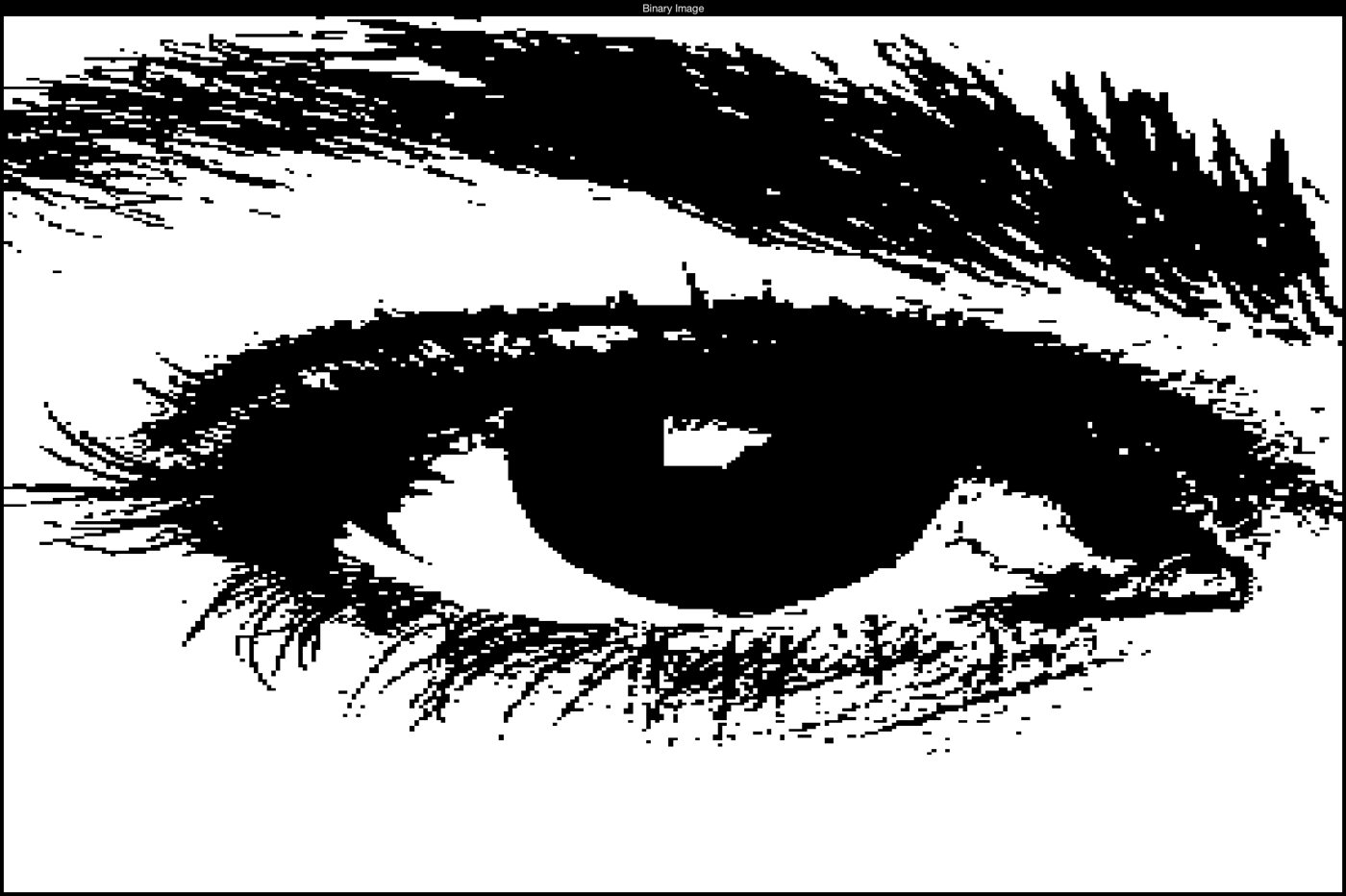
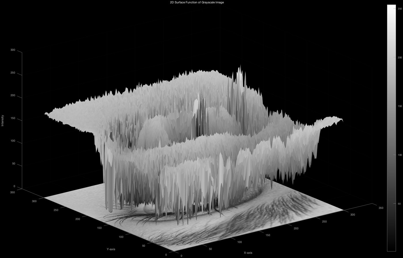
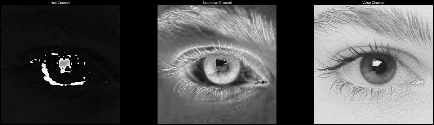
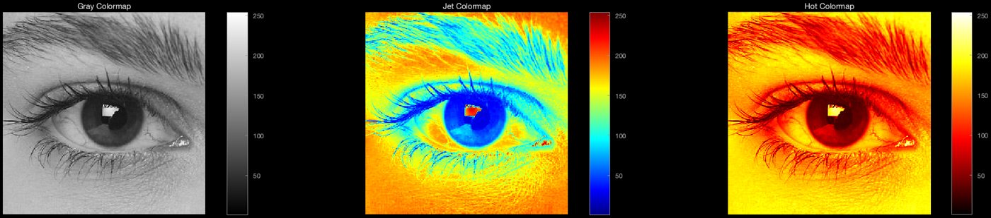
Working with a 300 × 300 uint8 close-up of an eye: reading metadata with imfinfo, saving it as TIFF, a manual grayscale average sum(img,3)/3, a 4-bit PNG and a PGM, then thresholding at the mean intensity and splitting it into HSV channels.
Pixels, regions & synthetic images
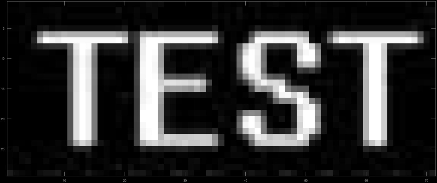
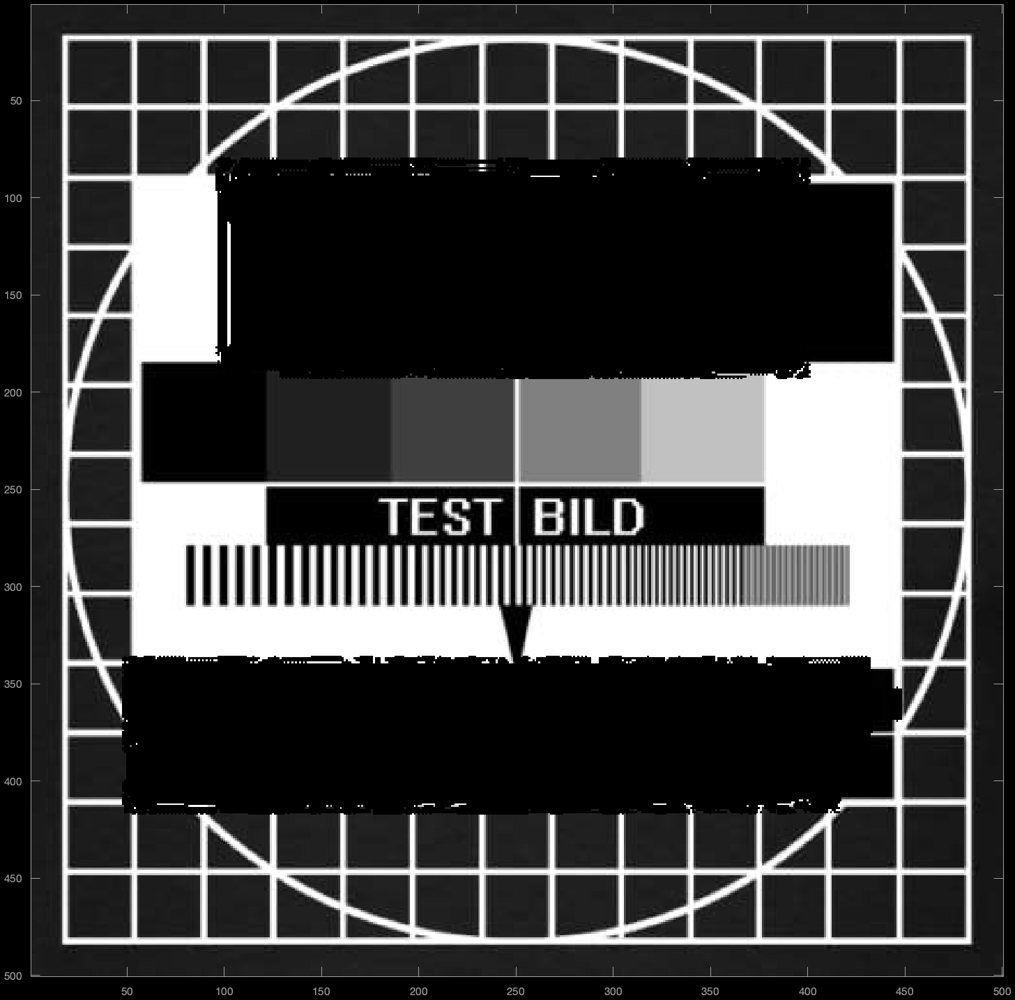
An image is a matrix. This set works on a TV test card: cutting out a region of interest by indexing img(250:278, 175:245, :), keeping only pixels where R == G == B, generating uniform and Gaussian noise images (μ = 128, σ = 50) and a bar pattern whose widths grow as k², and drawing shapes with insertShape.

Camera geometry
Pure linear algebra, no images: recovering a camera from its 3 × 4 projection matrix, then estimating a homography from four point correspondences. I wrote my own myInvK (cofactor inverse, no inv()) and mySkewMat helpers for it.
Decomposing P = K [R | t]
A QR decomposition of the flipped 3 × 3 block splits it into the upper-triangular intrinsics K and the rotation R. A sign matrix D = diag(sign(diag(K))) forces a positive focal length. The camera centre is the null space of P, the last right-singular vector of an SVD.
K   = [2000    0  600
          0 2000  800
          0    0    1]
T   = (-10, -10, 100)
O_w = (14.14, 70.71, 70.71)   % same from SVD and from -(KR)⁻¹KT
Homography with the DLT
Pixel points are normalised with K⁻¹. Each correspondence gives three equations [x]× (Xᵀ ⊗ I₃) h = 0, stacked into a 12 × 9 matrix A. The solution h is the last column of V from svd(A). The first two columns of H give the rotation, completed with a cross product and projected back onto SO(3) with another SVD.
R ≈ [0.709  0.503 -0.495
     0.705 -0.498  0.504
     0.007 -0.706 -0.708]
T ≈ (-9.99, -9.99, 99.89)   % matches the true T
Image enhancement & motion detection
The biggest set: geometric operations done by hand, intensity arithmetic, contrast stretching, gamma, statistics, histogram equalisation, and a live webcam motion detector. Drag the sliders to compare.
Rescaling a dark image
The dark flowerpots only use grey levels 0–211. Mapping that range to 0–255 lifts the whole image.


Gamma compression, γ = 0.5
255·(I/255)^0.5 brightens the shadows far more than the highlights. It matches imadjust(…, gamma).


Histogram equalisation
Bright flowerpots (mean 127.3, σ 51.5). histeq spreads the intensities over the full range.


Contrast spreading
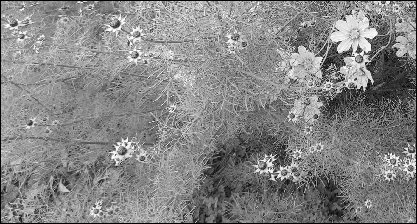
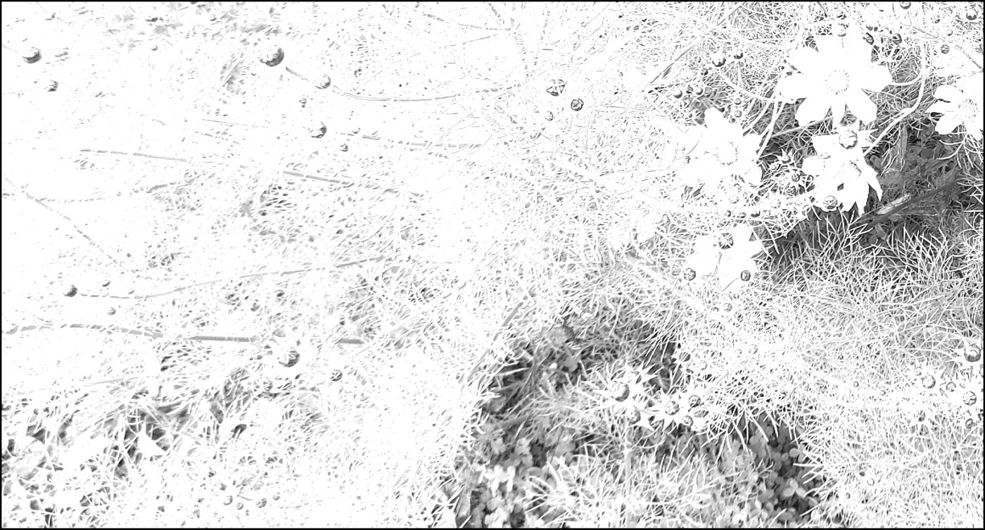
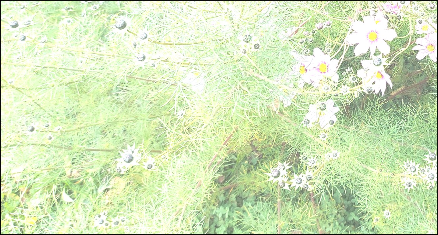
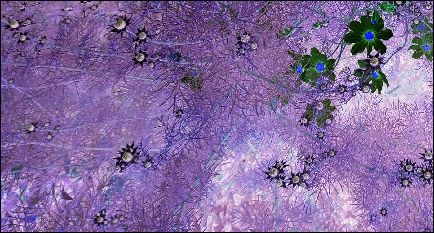
My contrast_spread(I, Gmin, Gmax) clips to a band and stretches it: here the dark half [0, 127] of the Cosmea image.


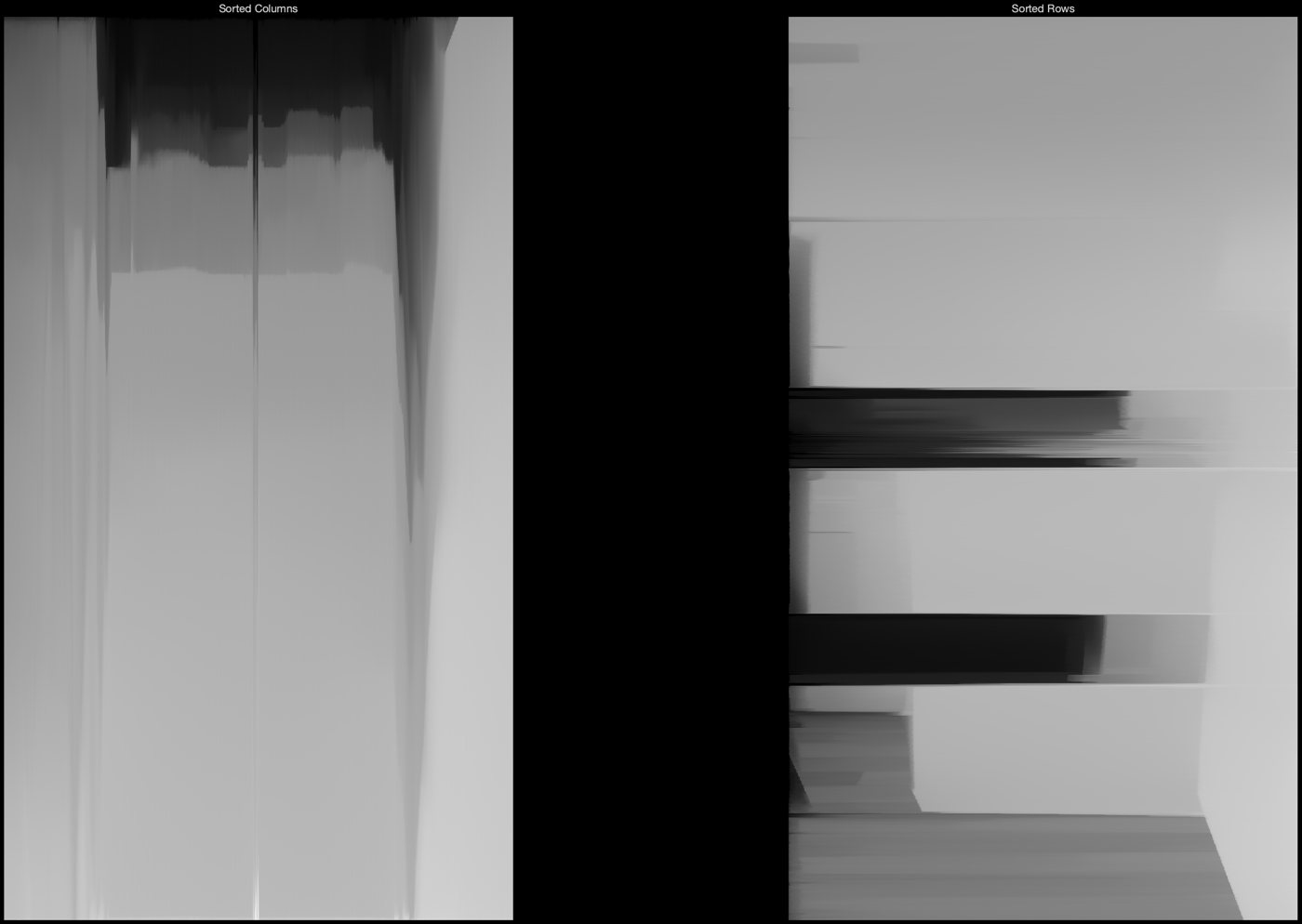
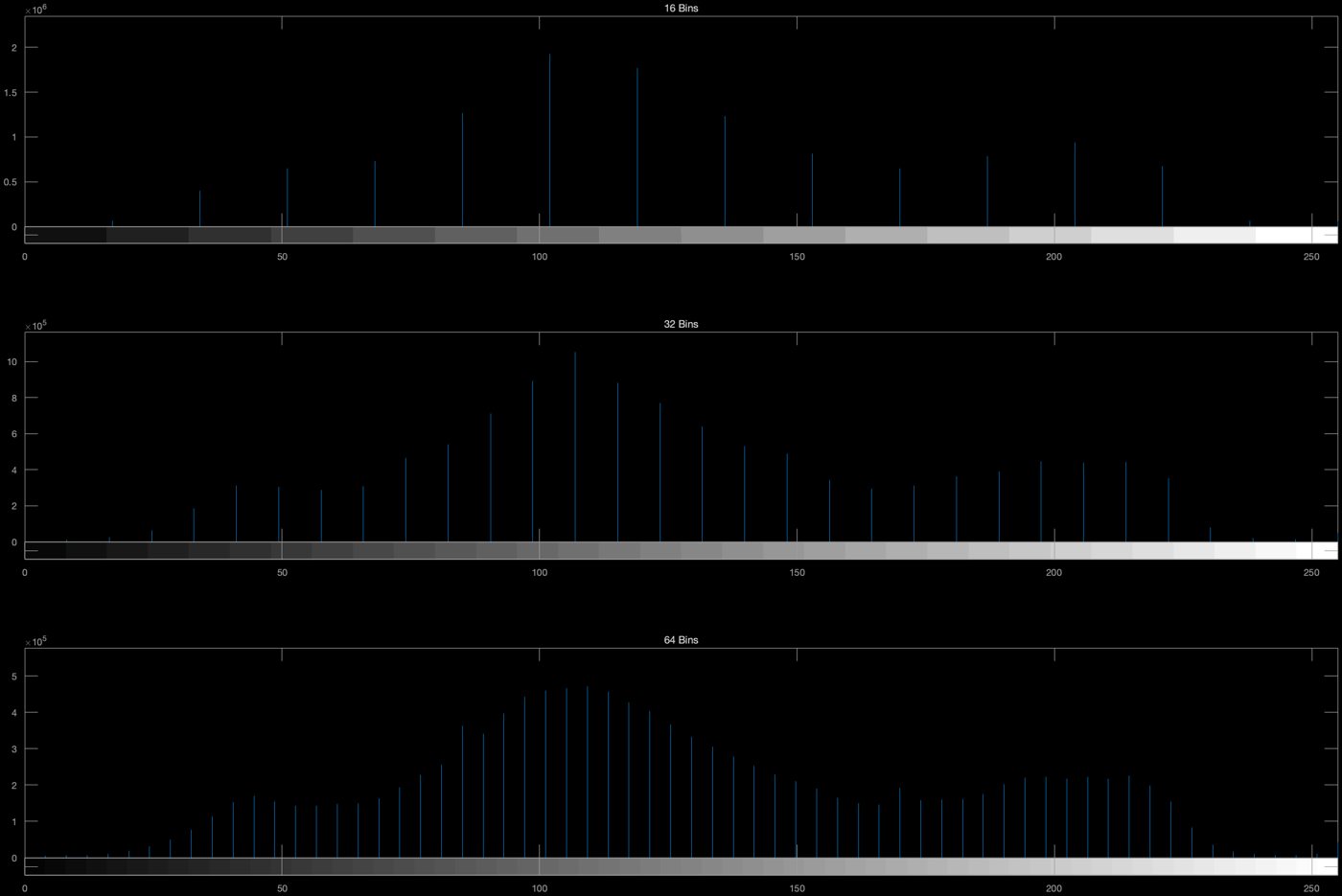
Statistics
After normalising to zero mean and unit variance, the autocorrelation comes out at exactly 1 and the cross-correlation with the negative image at −1, as the theory predicts.
Live motion detection
A webcam loop keeps an adaptive background H(t) = α·F(t−1) + (1−α)·F(t−2) with α = 0.5, computes the activity image |I − H| and thresholds it at τ = 30 to show moving silhouettes in real time. It needs a live camera, so there's no still here.
Fourier basis functions
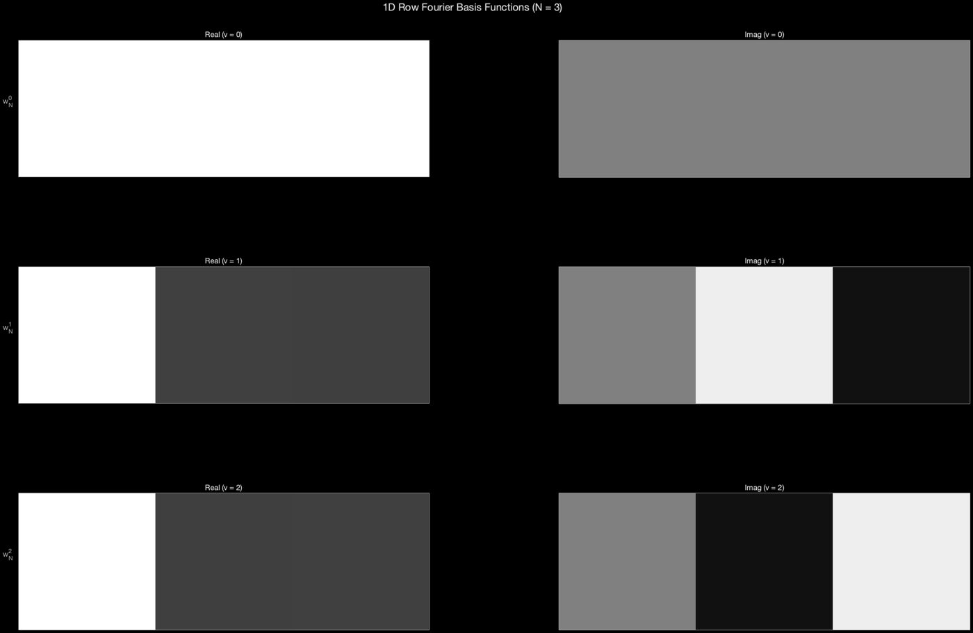
A 3 × 3 binary image is taken apart into its 1-D Fourier basis functions, computed in one vectorised line with Euler's formula exp(j·2π·v·n/N). The real and imaginary parts are shown for every frequency.
Fourier filtering & SVD
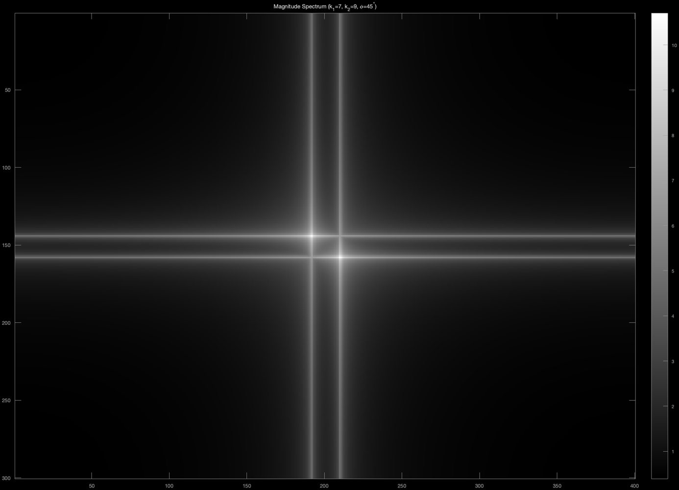
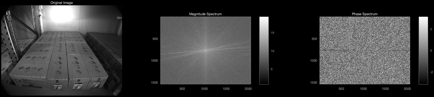
Two ways of taking an image apart. The 2-D FFT describes it as frequencies. A Gaussian weight in the frequency domain (σ = size/10) then keeps the low ones (blur) or, as 1 − W, the high ones (edges), before an inverse FFT rebuilds the image. The SVD describes it as a sum of rank-1 images ui·viᵀ.



Binary shapes
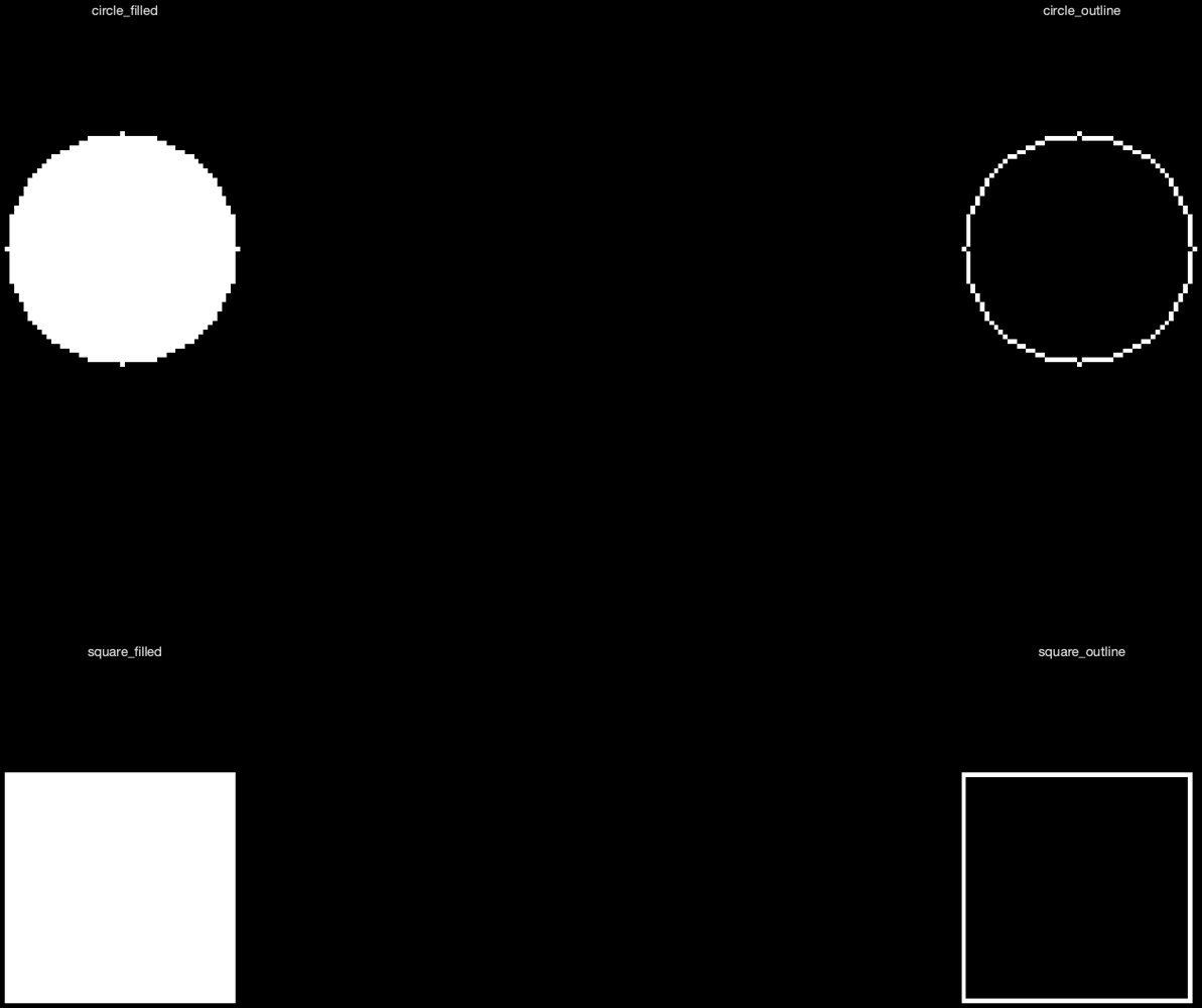
Shapes straight from their equations on a 100 × 100 grid: a filled circle is every pixel with hypot(X−cx, Y−cy) ≤ r, a square is an index range, and bwperim turns both into outlines. The masks are exported as PNGs.